Tag: education

  • Deep Bloom (Pt. 3)

    Oct. 26, 2026

    In Part 1, I compared shallow and deep understanding Levels 1 and 2 of Bloom’s Taxonomy (Knowledge and Comprehension, respectively, to use the original terminology).

    In Part 2, I did the same for Levels 3 and 4 (Application and Analysis).

    In this final installment, I do the same for Levels 5 and 6 (Evaluation and Synthesis).

    Note that the names of Bloom’s levels, as well as the order, are different depending on which version you’re looking at, but it doesn’t really matter.

    Level 5 (or 6): Evaluation

    Activities relating to using concepts to make judgments.

    Continuing with the example of the arithmetic mean, shallow understanding could be demonstrated by reliance on heuristics and decision rules.

    For example, when dealing with employee salaries, one might assume that the median is necessarily a superior representation of a “typical value,” because salaries tend to be positively skewed.

    But, as with all rules of this nature, it’s not so simple…

    Deeper understanding would take into account the nature of the particular situation or problem.

    For example, suppose the organization has narrow salary bands due to limitations by law or agreements with labor unions. If so, then the salaries might not be skewed much or at all! In that case, the median becomes no better than the mean (or possibly worse, depending on what you’re doing with it).

    It should not always be assumed that a variable must be distributed in a characteristic way (even if it usually is).

    Additionally, even if there truly IS positive skew, that doesn’t necessarily eliminate the relevance of the mean.

    For example, suppose you are analyzing compensation for a commission-based sales team. Imagine that most sales representatives on the team have comparable pay, but a few all-stars substantially increase their commissions year-after-year.

    • If you rely solely on the median to represent average team performance, this trend could be completely concealed.
    • But relying solely on the mean could lead to a different incorrect interpretation—that everyone on the team is improving, when it’s really just a few.

    Here’s a quick demonstration of this using R…

    > # Creating a toy dataset
    > typical=c(80,84,86,88,90,92)
    > stars=c(150,170)
    > (df=data.frame(id=101:108,
    + year1=c(typical,stars),
    + year2=c(typical,stars*2),
    + year3=c(typical,stars*4)))
    id year1 year2 year3
    1 101 80 80 80
    2 102 84 84 84
    3 103 86 86 86
    4 104 88 88 88
    5 105 90 90 90
    6 106 92 92 92
    7 107 150 300 600
    8 108 170 340 680
    > # The totals are increasing year after year...
    > colSums(df[2:4])
    year1 year2 year3
    840 1160 1800
    > # But the median does not reflect this!
    > (medians=apply(df[2:4],2,median))
    year1 year2 year3
    89 89 89
    > # The mean DOES reflect this...
    > # ...but it's biased by the all-stars!
    > (means=apply(df[2:4],2,mean))
    year1 year2 year3
    105 145 225

    The above demonstration shows that the median gives a more “typical” experience, whereas the mean reflects the overall group pay more accurately. That said, the latter is easily misunderstood; it paints a rosier picture than reality, because the change is only driven by a couple high performers.

    With a distribution this small, the solution might be simply to view all scores simultaneously, in a table or graph.

    For any number of scores, you could also combine the two types of averages to get a fuller picture…

    > # Ratio of mean/median year over year...
    > data.frame(medians,means,ratio=round(means/medians,2))
    medians means ratio
    year1 89 105 1.18
    year2 89 145 1.63
    year3 89 225 2.53

    The above table makes it clear that median pay is constant, while mean pay is rising (which suggests some subset of team members are getting increasingly higher pay).

    Again, what all this illustrates is that simplistic rules and heuristics like “Don’t use the mean when the distribution is skewed” are the domain of shallow understanding.

    Deeper understanding allows for considering what numbers are truly most relevant for a particular situation.

    Level 6 (or 5): Creation (Synthesis)

    Activities relating to combining concepts to create superordinate ideas or broader systems.

    Shallow understanding could be demonstrated by creating an HR analytics dashboard that includes various summary statistics for relevant variables, including means.

    Now, that’s not necessarily shallow. But it doesn’t inherently convey depth, either.

    With basic knowledge of key terms and formulas, as well as familiarity with coding or a platform like Tableau, this can be accomplished even by someone who has no idea whether the mean is relevant for the variables and situation at hand.

    One example of a task requiring deeper understanding is designing a job applicant scoring system that involves averaging ratings across a panel of interviewers, where it is known that one interviewer gives systematically harsher ratings than the others.

    At first blush, you might think that the more sophisticated approach would involve some kind of correction, like a trimmed mean. (In fact, I know a guy with a PhD who once suggested this solution to this exact problem.)

    This solution seems deeper, in that it doesn’t rely on canned statistical functions, and it takes into account the influence of skew…

    But in a typical selection system, the overarching goal is to rank-order applicants and make job offers to those highest-ranked.

    Critically, if a single rater is systematically more severe than other raters, this does NOT change the rank-order of applicants. (Assuming the same panel rates all interviewees.)

    This is because systematically lenient or severe ratings are like adding or subtracting a constant (on average) to each score, which “moves them” all in the same way, and therefore has no effect on rank.

    Consequently, you don’t need to make any adjustment at all! You can preserve all the information that the panel members provided about the applicants—and therefore avoid inflating average scores—while still getting the same applicant rankings.

    Here’s a quick demonstration in R …

    > # Creating a dataset of job applicant ratings
    > (ratings=data.frame(
    + Candidate=c('Applicant A','Applicant B','Applicant C','Applicant D'),
    + Rater1=c(4,3,5,2),
    + Rater2=c(5,3,4,2),
    + Rater3=c(4,4,5,1),
    + Rater4_harsh=c(2,1,3,0)))
    Candidate Rater1 Rater2 Rater3 Rater4_harsh
    1 Applicant A 4 5 4 2
    2 Applicant B 3 3 4 1
    3 Applicant C 5 4 5 3
    4 Applicant D 2 2 1 0
    > # Rater 4 is systematically harsher than others
    > # Rank-ordering applicants
    > rank(rowMeans(ratings[,2:5]))
    [1] 3 2 4 1
    > # Rankings without the harsh rater
    > rank(rowMeans(ratings[,2:4]))
    [1] 3 2 4 1
    > # The rankings are unchanged...

    This shows that corrections like trimming extreme scores (in this case, literally eliminating the harsh rater’s scores from the dataset) have no effect on the actual applicant rankings.

    And I can tell you from experience that this is far from obvious to most people, including many who have taken multiple statistics courses.

    Now, this is not to say that corrections would never be appropriate. The point is just that choosing the right solution requires deep conceptual understanding of how averages like the arithmetic mean work.

    Real-world applications require greater depth of understanding than mere definitions, formulas, and canned code.


    All right, that’s all six levels. Hopefully I’ve made it painfully clear that depth of understanding does NOT necessarily rise along with successive levels of Bloom’s Taxonomy.

    A reasonable question at this point might be, “Okay, so exactly how deep should we expect a given student’s understanding to extend?”

    And I guess the answer must be individualized to the learner, instructor, training curriculum, university, and/or other context.

    More generally, How deep does anyone’s understanding need to extend?

    As I’ve mentioned previously, it’s relatively easy to identify shallow understanding, as well as to distinguish shallow from deep…

    But it’s never clear how deep deep can be. How far down the rabbit hole can you go? Does it ever bottom out?

    I don’t know. For now, I’ll keep digging.
  • Deep Bloom (Pt. 2)

    Oct. 25, 2026

    Part 1 compared shallow and deep understanding for the first two levels of Bloom’s Taxonomy. This post covers the next two levels, again using the mean (average) as the example.

    Level 3: Application

    Activities relating to using concepts to solve novel problems.

    Shallow understanding at this level would involve simply plugging numbers into an algorithm to produce the mean.

    For example, I might use the following R code to find the mean for the values (1, 2, 3, 4, 5, 6).

    > mean(1:6)
    [1] 3.5

    Clearly, this shows one can apply some superficial concept of the mean (e.g., “it’s an important number I can get with the mean() function”) to solve novel problems without necessarily having any idea what it actually means.

    A contrived problem like this could be made trickier to test deeper understanding.

    For example, suppose that a class of 24 students has an average exam score of 85, and a separate class of 31 students has an average score of 82. What’s the average score across the two classes?

    Without grasping the underlying concept, the first thought might be to average the averages: (85 + 82)/2 = 83.5.

    But this is WRONG.

    As mentioned last time, the arithmetic mean can be conceptualized as an equal share per unit. In other words, if we totaled all the scores in the distribution, then cut the total into equal parts, the size of each equal part would be the mean.

    But the combined classes do NOT have 2 scores, so that’s the wrong denominator; the combined count is 24 + 31 = 55. We need to account for that in our calculation.

    (There’s a quick formula to solve for a weighted mean, but going straight to that from memory would again be missing the point here. That approach could also be employed formulaically, without really understanding what’s going on at a conceptual level.)

    If we had all the individual scores, we could just ignore the individual class means and calculate the overall. But since we only have summary data, we’ll have to reverse-engineer it…

    The mean for one class is found with M₁ = Σx₁/n₁. That means that we could multiply the mean times the count to get total: Σx₁ = M₁n₁. We can do this for both groups… Σx₁ = 85 ⋅ 24 = 2040 and Σx₂ = 82 ⋅ 31 = 2542.

    Now we can find the total sum and the total count for the two groups combined: Combined Mean = (Σx₁ + Σx₂) / (n₁ + n₂) = (2040 + 2542) / (24 + 31) ≈ 83.31.

    In fact, the process we just walked through can be formalized as Weighted Mean = (M₁n₁ + M₂n₂) / (n₁ + n₂). This is the quick formula I mentioned previously, but, again, simply memorizing it would bypass the underlying intuition.

    If someone genuinely understands the concept of the mean at a deep level, then they could figure this out on their own, without needing to be taught the formula separately.

    Level 4: Analysis

    Activities relating to breaking concepts down into sub-components.

    Shallow understanding, at the most basic level, would involve simply recognizing and grasping the two components of the mean formula:

    1. The sum of the values, Σx
    2. The number of values, n

    It might follow from this that outlying values can drag the mean around, which might constitute deeper learning. But there is also a version of such “understanding” that is merely a memorized rule: The mean is dragged in the direction of outliers.

    If someone told me that, I’d be tempted to ask, “Why? What makes it work that way? Does this happen in some lawful way?”

    And those are harder questions to answer…

    Deeper understanding could come from examining the formula more closely…

    The formula Σx/n could be rewritten as x₁/n + x₂/n + … + xₙ/n. This provides an alternative interpretation of the mean as a weighted sum of scores, where each score gets a weight of 1/n (meaning each score counts equally).

    As such, each score contributes xᵢ/n to the mean. That is, every score contributes in proportion to its own value (but the influence is scaled by the total number of scores).

    This is why every score (including outlying values) “pulls the mean” in its own direction. The further a given score, xᵢ, lies from the other values, the more it changes the mean from what it would be without xᵢ.

    To illustrate this, let’s see what would happen if we changed the value of a single score…

    Increasing a given score by Δ increases the total sum of the distribution by exactly Δ. Therefore, taking the weight (1/n) into account, the mean must increase by Δ/n.

    For example, consider this set of scores: (0, 1, 2, 3, 4). If we increase that first value from 0 to 500 (i.e., Δ = 500), it will increase the total sum by 500, and it will increase the mean by Δ/n = 500/5 = 100.

    Here’s a quick demonstration in R…

    > # Create a distribution with 5 scores...
    > x=c(0,1,2,3,4)
    > sum(x)
    [1] 10
    > mean(x)
    [1] 2
    > # Increase the first value by 500
    > x[1]=x[1]+500
    > # Now the sum has increased by 500...
    > sum(x)
    [1] 510
    > # And the mean has increased by 500/5 = 100...
    > mean(x)
    [1] 102

    (We would also see the opposite pull downward if Δ were negative.)

    But, by the same token, this also demonstrates how the extent of any single value’s influence is controlled by the number of scores.

    In the above example (n = 5), the Δ for that first score changed the mean dramatically. But if we have 50,000 scores, the same increase has almost no effect…

    > # Create a distribution with 50k scores...
    > set.seed(123)
    > x=sample(1:5,50000,T)
    > sum(x)
    [1] 150075
    > mean(x)
    [1] 3.0015
    > # Increase the first value by 500
    > x[1]=x[1]+500
    > # Now the sum has increased by 500...
    > sum(x)
    [1] 150575
    > # But the mean has only increased by 500/50000 = .01...
    > mean(x)
    [1] 3.0115

    In this way, all values in the distribution “drag the mean around,” but this influence is most apparent when (1) a given score is further away from the others and (2) there are relatively few datapoints in the distribution.

    And this is just one example of how breaking the concept down into component parts could lead to a deeper understanding—in this case through rearranging the formula to get a different intuition.


    Okay, once again, this ended up being longer than expected. Final installment tomorrow…

  • Deep Bloom (Pt. 1)

    Oct. 24, 2026

    In a previous post, I gave examples of how a person could understand the mean (average) across all six levels of Bloom’s Taxonomy.

    But I later argued that Bloom only gives us categories of activities relating to knowledge, not necessarily levels of increasing complexity or depth.

    To more clearly illustrate what I mean, below are examples of both shallow and deeper understanding at each level of Bloom…

    Level 1: Remembering (Knowledge)

    Activities relating to identifying and recalling concepts.

    Sticking with the example of the mean (average)…

    Shallow understanding can be demonstrated by writing out a basic version of the formula, Σx/n, or saying something like, “Add up the parts, then divide by the number of parts.”

    While this is accurate, a person could write or utter these words without necessarily being able to clarify what any of it actually means.

    Deeper understanding in this level might constitute memorizing a network of concepts within which the mean sits.

    For example, you might know that this is only one type of average among many, including…

    • Mean
    • Median
    • Mode

    In fact, it’s not even the only mean out there. This category includes…

    • Arithmetic mean (what people usually mean by “average”)
    • Geometric mean
    • Harmonic mean

    At this level of Bloom, deeper understanding could include the ability to identify and recall definitions and formulas for each of these and others.

    It could also include knowing different or more complex variations of the formula, which type of average is most appropriate for different types of analytic situations, and so on…

    Ultimately, however, all these terms, as well as their definitions and formulas, are just words, which are merely labels for concepts.

    As such, while it would be difficult to imagine someone having deep understanding of these concepts without knowing the relevant terms, that knowledge alone is still not sufficient to guarantee comprehension.

    Imagine you memorized a brief passage in a foreign language by writing and speaking it daily…

    At some point, you’d have it down pat. But unless you ever bothered to translate it, you’d never know what any of it meant!

    In the same way, a person could memorize every relevant term and definition in a given subject domain until they could recite it all at will, and that still wouldn’t guarantee that any of it meant anything to them.

    Level 2: Understanding (Comprehension)

    Activities relating to explaining concepts.

    Shallow understanding here might be demonstrated by an explanation like, “The mean is a typical or average score in a distribution.”

    This is true, but it’s incredibly vague. It seems to overlook the existence of other types of averages (see previous section). There’s also no apparent realization that certain factors (e.g., outliers, distribution shape…) could affect how well it typifies the distribution.

    Two common candidate explanations for deeper understanding would be…

    1. The mean as the balancing point of the distribution; half the “weight” lies below it, and half lies above it. This is why the sum of deviations from the mean is always zero.
    2. The mean as the equal share per unit; if we totaled the scores, then cut the total into equal parts (one for each observation in the distribution), the value of each part would be the mean.

    This is usually how I introduce the concept to students.

    But we could go even deeper.

    Perhaps the deepest (?) level of any mathematical or statistical concept is the algorithmic level.

    Here’s the idea: If you truly understand a concept, you should be able to create your own algorithm from scratch that reproduces the idea. (Doesn’t really matter whether it’s unique or not, so long as you generate it yourself.)

    One way to take the arithmetic mean to this level of understanding is to realize it’s only one case of a more general process. There are more technical versions of this, but here’s the basic generalization…

    Suppose you perform some operation (e.g., addition, multiplication) on a set of values, resulting in a total effect. For example, summing all the values results in a total; multiplying all the values results in a product; et cetera.

    A mean is a single value that could replace each score in the distribution without changing the result of that operation.

    Consider summation (adding things up)…

    If our set of scores is [1, 2, 3, 4], the result of summation would be 1 + 2 + 3 + 4 = 10. The arithmetic mean, Σx/n = 2.5, is the only value that could replace each score in that operation, while still producing the same result: 2.5 + 2. 5 + 2. 5 + 2.5 = 10.

    Or consider multiplication…

    The product of multiplying all the values in that same distribution is 1 ⋅ 2 ⋅ 3 ⋅ 4 = 24. Again, the geometric mean, ⁿ√(Πx) ≈ 2.2134, is the only value that could replace each score in that operation, while producing the same result: 2.2134 ⋅ 2.2134 ⋅ 2.2134 ⋅ 2.2134 ≈ 24.

    What makes this explanation “deeper”?

    To me, it’s deeper in that it represents a more general principle about how things work. The mean is not (just) an arbitrary concept that people use by convention; it fits into the bigger picture of how math works.

    Based on this, it becomes apparent that there are infinite number of possible means that we could define.

    This allows for understanding an entire class of calculations with a single concept. For example, someone who understands the above explanation is in a far better position to next grasp the harmonic mean and various other means.

    Viewed through this lens, the arithmetic mean is only one case of a single value that can represent a distribution of scores in a particular context. It’s not some magical statistic that we should always default to when summarizing a set of scores. (This has critical implications for other Bloom levels, like application, creation, etc.).

    Another takeaway from this discussion is that deeper understanding can often be acquired by exploring different ways of explaining the same concept.

    The more multidimensional your understanding of a concept, the more your mental representation of it begins to transcend any particular set of symbols on a page.

    And it doesn’t have to stop here.

    Yet another alternative explanation could be through a regression lens:

    Using an ordinary least squares approach, the arithmetic mean is the predicted value of the distribution when no additional variables are taken into consideration (i.e., no predictors; intercept-only model).

    By “predicted value,” I mean one possible “best guess” for what a randomly selected score from the distribution would be.

    And on and on it goes…


    Okay, this post is already longer than I expected it to be. More next time…

  • What’s Wrong With Flowcharts and Decision Rules in Statistics Education?

    Oct. 23, 2026

    Last time, I gave a fictional (though in one sense very real) example of a person who has demonstrated learning/understanding of statistics in each level of Bloom’s Taxonomy, despite not truly understanding the subject in much depth.

    In one sense, this person is certainly accomplished, in that they have completed all the steps necessary to be awarded a graduate degree. It probably even took a lot of hard work and energy over multiple years.

    But if the entirety of someone’s knowledge in a subject boils down to key terms, written procedures, and decision rules, it’s debatable whether we could really say they “understand” what’s going on.

    It would be like charting the surface area of a lake but never looking underwater. The vast majority of the lake’s characteristics exist below the surface.

    (By the way, this kind of education really does happen, and sometimes such individuals go on to become statistics educators! And then the cycle continues.)

    What’s the problem with flowcharts and decision rules?

    There’s nothing inherently wrong with them. But the fundamental reason that statistics educators teach them is to avoid having to explain what’s really going on.

    Two possible reasons for this include:

    1. Statistics educators themselves don’t understand beyond the flowcharts and decision rules.
    2. Statistics educators do understand more deeply, but they don’t believe their students are capable of deeper understanding.

    For example, consider the hotly debated p-value…

    Many instructors simplify the concept to something like, “If this value is less than .05, then the research hypothesis is supported” (a semi-arbitrary decision rule).

    If they’re teaching the concept like this, it’s also highly unlikely they’re explaining how to calculate p-values; more likely, they’re teaching how to click buttons to make the p-value appear.

    So the learning ultimately boils down to instructing the computer to do something for you, then making conclusions about the nature of reality based on what shows up on the screen.

    I knew one stats instructor who actually said, “If you see p < .05, then it’s time to celebrate! We got what we wanted!”

    This reflects such a profoundly confused understanding of not only statistics but science more broadly that I’m almost at a loss for words. Almost.

    So why do many educators avoid giving the true explanation for p-values?

    Because the true answer is much harder to explain and understand!

    The simplest accurate version would be something like, “Imagine the focal effect is literally zero*. If we ran this exact study an infinite number of times and plotted all the resulting test statistics, they would pile up like this [indicate a plot with the appropriate null sampling distribution]. Then we find where our actual observed test statistic lies in this distribution. The p-value is the proportion of area under this curve which is at least as extreme as our observed statistic. So it represents the probability we’d see a result at least as extreme as ours if the true effect were literally zero. This gives us some sense of how plausible the null hypothesis is.”

    (*Note that this explanation assumes the null hypothesis is the nil hypothesis [i.e., the effect is 0]. We could actually use any null we wanted in a significance testing framework like this.)

    I can assure you from experience that even highly intelligent people need that concept explained to them repeatedly and with multiple visuals before they start to develop some intuition for it.

    But once you do understand, then you almost become unable to interpret the result according to an arbitrary decision rule like, “If p < .05, reject the null hypothesis.”

    Someone who genuinely understands can only see a p-value for what it truly is: A piece of information about what the world looks like if X is true, which therefore also serves as evidence regarding the plausibility of X.

    Decision rules like α = .05 exist for people who don’t understand the underlying concepts well enough to make their own judgments.

    Flowcharts and decision rules exist to help us avoid understanding.

  • Levels of Bloom’s Levels

    Oct. 21, 2026

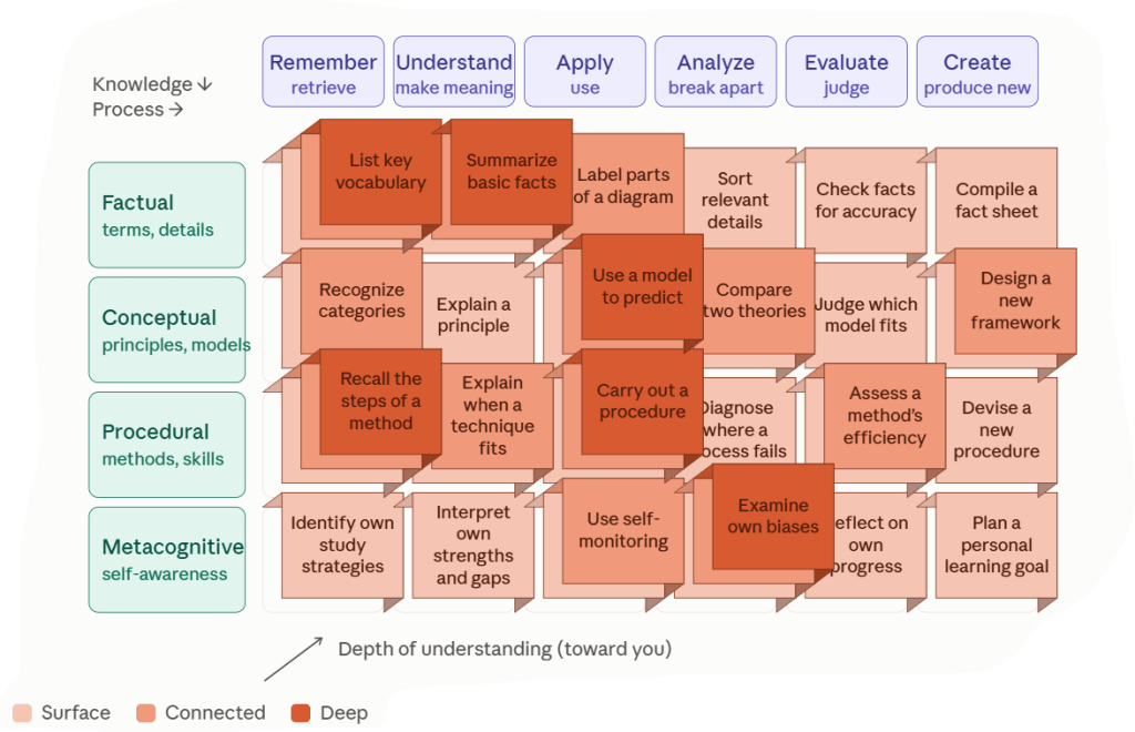
    You might think that Bloom’s Taxonomy makes the concepts of learning or understanding complicated enough, but the model is actually more complicated than I previously let on—and I would argue that the reality is even more complicated than the full model suggests!

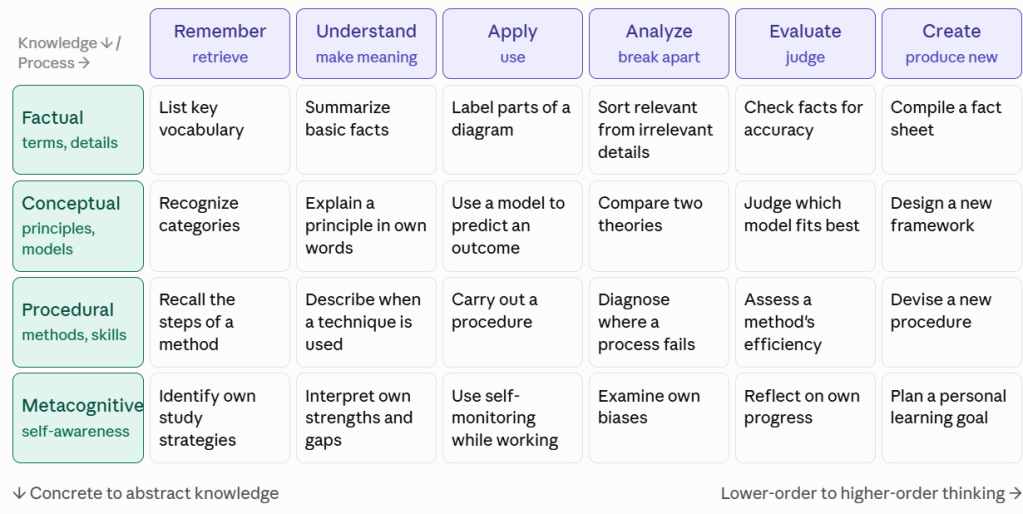
    Here’s the 2001 revision of the model, which still breaks learning down into 6 levels of generally increasing complexity…

    1. Remembering
    2. Understanding
    3. Applying
    4. Analyzing
    5. Evaluating
    6. Creating

    If you’re paying attention, you’ll notice that the 5th and 6th levels are swapped in the revised version. Additionally, the levels are now framed as verbs. (This is due to how educators write learning objectives, which is one of the primary uses of the taxonomy.)

    Previously, I described the levels in a general “overview” way. In actuality, scholars have broken down each of the six levels into sub-components. For example…

    • Remembering breaks down into identifying and recalling (think “matching” vs. “fill-in-the-blank” test questions).
    • Understanding breaks down into several dimensions, including classifying, comparing, explaining…
    • Evaluating breaks down into checking and critiquing.
    • Et cetera

    Additionally, the different levels can be mapped against different types of knowledge (e.g., factual vs. procedural).

    Here’s a 2D representation of this idea, with example tasks in each cell (courtesy of Claude):

    (For details on the actual revised model from the scholars themselves, check out Anderson & Krathwohl [2001].)

    But even within this more nuanced framework, I would argue that there are degrees of understanding at each level and its component dimensions, on a spectrum from shallow to deep.

    For example, in the Remembering/Knowledge level, consider a person’s recall of facts in a subject area. Their extent of recall could be…

    • Shallow (e.g., remember a few introductory key terms)
    • Deep (e.g., remember many advanced terms)
    • Or anywhere in between

    Or in the Understanding/Comprehension level, consider a person’s ability to explain some mechanical process, such as how a lightbulb works. Again, their extent of explanatory ability could be…

    • Shallow (e.g., vaguely describe the general process)
    • Deep (e.g., describe the process in great depth and in multiple ways)
    • Or anywhere in between

    This is called explanatory depth.

    I’m not the only person who has thought of this, by the way. For example, Biggs & Collis (1982) published a model of what is essentially depth of learning, which they map onto cognitive developmental stages.

    Additionally, the concept of explanatory depth is the subject of an entire research literature—the illusion of explanatory depth (i.e., the study of how we typically LACK the ability to explain causal processes with as much depth as we think we can).

    It doesn’t look as clean, but I had Claude add a third dimension to the previous image to represent depth of understanding. (Appropriately, if the other two axes represent length and height, then this third dimension represents literal depth.)

    This is an attempt to illustrate how different demonstrations of knowledge can occur with varying amounts of depth; therefore, it is not as simple as higher-order processes always representing greater depth of understanding.

    (Granted, I suspect that higher-order levels such as Creating generally do correspond to deeper understanding than lower-order levels such as Remembering; my argument is only that it’s not guaranteed.)

    In this way, I view Bloom’s Taxonomy merely as six types of activities relating to knowledge. This argument doesn’t make the framework any less useful, but it does reveal a clear problem…

    A person could technically demonstrate “understanding” in all six of Bloom’s levels while still having basically no idea what they’re talking about.

    Reflecting on my own learning process, as well as what I observe in others, it seems to me that “shallow mastery” is more common than we’d like to believe, and it’s far less common than deep understanding.

    More on this next time…

  • Levels of Understanding

    Oct. 20, 2026

    What does it mean to understand something?

    The question, “How do you know if you understand something?” proves surprisingly difficult to answer. The more you grapple with it, the less it even seems like a sensible question to ask.

    Perhaps it’s better to conceive of understanding NOT as a binary classification (i.e., one either does or does not understand) but rather in terms of degrees (i.e., one understands to what extent and in what ways).

    An extremely popular model of levels of understanding is Bloom’s taxonomy, which outlines 6 levels of learning or understanding…

    1. Knowledge—Identifying concepts
    2. Comprehension—Summarizing related concepts
    3. Application—Using concepts to solve problems
    4. Analysis—Breaking down related concepts to explain how they are connected
    5. Synthesis—Building superordinate ideas by combining concepts
    6. Evaluation—Making judgments based on understanding of the concepts

    Sometimes there are different variations of these terms, definitions, or order, but it doesn’t really matter.

    (As an aside, it’s always popular for people to argue about the validity or structure of popular models like this, but I think it’s mostly a waste of time. There is no “official” or “complete” framework of such categories.

    This framework is simply one way to think about more or less advanced levels of understanding.)

    Let’s take a basic example from data analysis: the average (what in statistics we call the arithmetic mean)…

    1. Knowledge

    Demonstrating knowledge might include writing down the formula…

    M = Σx/n

    Often, when I ask students what the “mean” is, they say something like, “Add up the parts and divide by the number of parts.” (A verbal statement of the formula.)

    This is 100% correct, but that is often the extent of most people’s understanding.

    When I ask…

    • “And what does that mean?”
    • “Why would we add up the parts and divide by the number?”
    • “What does the result tell us?”

    …I am usually met with silence.

    This might reflect that they have only memorized some surface-level features of the concept in a pattern-matching way.

    Or it’s possible that they do understand at a deeper level, but they’re less confident in that explanation, so they’re reluctant to put themselves out there in front of the class and risk embarrassment.

    Either way, their grasp is limited in some sense.

    A deeper level of understanding is represented by…

    2. Comprehension

    Demonstrating comprehension might involve expressing the concept in your own words…

    For example, here’s the explanation of the mean that pops into my head in this moment:

    “The arithmetic mean is a single summary value intended to represent an entire collection of scores. It is equivalent to taking the total of the scores and slicing it into equal-sized parts, which gives some sense of what the ‘typical’ score looks like.”

    There are other (better) definitions out there, but this is not a bad one.

    The only way I’m able to articulate this on the spot is that I have some sense of the concept in my mind, beyond a memorized definition.

    To me, this description carries more explanatory power than reciting the formula alone does.

    Without this deeper level of understanding, it’s not really clear why you would ever bother to calculate the mean in the first place!

    3. Application

    Applying the concept might involve using it to solve a real-world problem…

    Suppose a new worker is completing a series of four online safety training modules, and they need an average quiz score of 80% to pass. If their scores so far are 75, 90, and 85, what minimum score do they need on the final quiz in order to pass?

    There are many ways to find the answer, but one is to treat it as an algebra problem that uses the formula and an unknown…

    (75 + 90 + 85 + x) / 4 ≥ 80

    Solving for x yields…

    x ≥ 70

    They need at least a 70% on the final quiz to pass. Since the employee has never scored that low on a quiz so far, their odds seem good!

    4. Analysis

    Analysis involves breaking the concept down. Analyzing the mean might involve taking apart the formula and examining the implications of each part’s inclusion.

    For example, the arithmetic mean boils down to totaling the scores (Σx) and dividing by the number of them (n).

    Because every score (x) contributes to the total (sum, Σ), one implication is that any single value could be highly influential in determining the final result.

    Consider these two example distributions, which are identical except for their final values…

    A = (1 2 3 4 5)

    B = (1 2 3 4 500)

    Here are the mean calculations in R…

    > A=c(1,2,3,4,5)
    > paste('The mean of A is',mean(A))
    [1] "The mean of A is 3"
    > B=c(1,2,3,4,500)
    > paste('The mean of B is',mean(B))
    [1] "The mean of B is 102"

    The average is over 30 times larger in the second case. Clearly, a single datapoint can have a substantive impact on the mean.

    This seems obvious once you consider how every single score is contributing to the total, but it’s not obvious to most people who only have a vague grasp of what an average really is.

    5. Synthesis

    In some ways, synthesis is the opposite of analysis (going the other direction), because rather than breaking things down, we are building things up.

    To me, this often seems like a more creative version of application…

    For example, imagine an employee listening team is monitoring morale with pulse surveys randomly sent out to different segments of the workforce daily. To make sense of and use the data, they might synthesize the insights to create some kind of reporting protocol.

    For instance, perhaps they average scores to an engagement item daily (application). But they notice that scores are lower on Monday and higher on Friday (analysis), so they proceed to average the daily scores into weekly scores.

    Then, perhaps they notice random spikes up or down on certain weeks (analysis), which detracts from the overall picture of how engagement is progressing. So they begin calculating rolling 3-point averages to smooth out the jaggedness in the overall trend.

    In this case, the output (maybe some kind of dashboard) is a combination of many components, including some averages and variants of averages.

    6. Evaluation

    Demonstrating the ability to evaluate could involve making judgments that involve understanding of averages.

    For example, suppose a corporate firm reports that their average (mean) annual salary is $140,000 companywide.

    Someone who understands that the mean is dragged in the direction of outliers would (hopefully) immediately recognize that this average pay level could reflect that everyone in the firm makes about that amount…

    …or it could just as easily reflect low pay in general, combined with astronomical pay for a handful of C-suite executives.


    I have my own quibbles with Bloom’s Taxonomy (including the revised version, which I didn’t mention), but overall it’s a useful way to think about different levels of depth in understanding that are possible.

    But even within a given level, there can exist shallow versus deep understanding…