Nov. 3, 2026

Last time, I explained how I think about p-values, which only partly aligns with the classical null hypothesis significance testing paradigm. (In brief, I view a p-value as a graded piece of information, NOT as a binary indicator of “statistical significance.”)

This time, let’s see if we can represent this concept using R code. If the representation is accurate, then the results of our custom code should match the results of a standard analysis using canned R code from existing packages.

First, let’s simulate some data for two variables…

> # Generating Random Data
> set.seed(123)
> x=rnorm(500,100,15)
> y=x*2+rnorm(500,sd=160)

I know these two sets of scores will be correlated, because I directly defined the second set (y) based on the first (x), with some random noise added in.

Next, let’s correlate the two sets of scores and save that as “r”…

> # Checking the Correlation (r)
> (r=cor(x,y))
[1] 0.1276118

Okay, so there’s a correlation of r ≈ .128.

But what is the p-value for that r? Let’s check…

> # Extracting the p-Value from a Significance Test
> (p=cor.test(x,y)$p.)
[1] 0.004262684

This correlation is associated with p ≈ .004. (That symbol is the Greek letter rho, by the way, NOT p.) This p-value means that, if the true effect were precisely ρ = 0, then we’d observe an effect at least as extreme as r = .128 only .4% of the time (i.e., about 4 times in 1000).

That’s not very often. One might suggest that this is relatively unlikely if the null is true…in which case, perhaps the null is UNtrue…

More information would need to be taken into account, but, all else being equal, a smaller p-value may be interpreted as evidence against the null hypothesis that there is zero effect.

(Remember the signal detection logic from last time.)

((Also, if that claim just triggered you, then go read my previous post on this topic. I define “evidence” as any piece of information that sways your credence toward a particular belief. If you’re feeling agitated, it’s probably because you are defining “evidence” differently.))

Also Note: I don’t need to check the statistical assumptions in this particular case, because I defined the two variables so that the assumptions would be met.

Next, let’s walk through the process of creating a null distribution (a pile of results that would be expected if the true effect were literally zero).

There are more elegant ways to do this, but I’m going to use brute force, because this approach is easier for me to understand (which is the entire point)…

Below, I’ll simulate 1 million independent pairs of distributions—meaning the true correlation between each of them MUST be nothing (i.e., ρ = 0)—and then I’ll correlate them all. The pile of correlations will serve as our null distribution.

# Simulating 1 million pairs of unrelated datasets
set.seed(1234) # For reproducibility
sim_rs=replicate(1000000,cor(rnorm(500),rnorm(500)))

It is important that n = 500 for each simulated dataset, because that’s the size of our “observed data” from before.

On my device, the above code took about 1 minute to run.

Before calculating the p-value, let’s visualize this null distribution…

# Plotting the Null Distribution
plot(density(sim_rs),xlim=c(-.3,.3),
     xlab='',ylab='',main='')
abline(v=r,lty=2,lwd=2,col='blue')

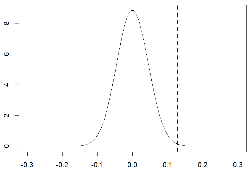
I drew a blue dashed line to represent where our original observed statistic (r = .128) lies in this null distribution.

Now, remember that the p-value is the proportion of this distribution that is at least as extreme as r = 1.28 (whether positive or negative).

We can calculate that using this R code…

> # Calculating an empirical p-value...
> mean(abs(sim_rs) >= abs(r))
[1] 0.004167
> # Compare to the p-value that cor.test produced...
> p
[1] 0.004262684

Our simulation produced an approximation (p = .004167), which is pretty close to the more precise value calculated earlier (p ≈ .004263).

The reason it’s not even closer is that I “only” used 1 million pairs of distributions in the simulated datasets.

If we want our approximation to be even closer, we could simulate, say, 10 million pairs of datasets.

I did it so you wouldn’t have to (took about 10 minutes on my device)…

> # Simulating 10x more data
> set.seed(1234)
> sim_rs=replicate(1e07,cor(rnorm(500),rnorm(500)))
> # Calculating an empirical p-value
> mean(abs(sim_rs) >= abs(r))
[1] 0.0042553
> p
[1] 0.004262684

The two calculations would only continue to converge as we increased the number of pairs of simulated datasets.

Okay, that does it for the demonstration.

As we can see, our conceptualization of what a p-value is and where it comes from DOES seem to align with results that are produced from mathematical theorems (at least to an approximation).

Again, the interpretation of a given p-value is still up to the individual. As can be seen from the graph above, a correlation this extreme is fairly surprising in this null distribution. But it certainly doesn’t seem unfathomable by any stretch, at least not in my opinion…

At the risk of belaboring the point, this demonstration reveals another intuitive way to think about significance tests…

They ask, “Is the effect far enough away from zero, relative to the amount of noise in the data, that it seems like more than mere noise?”

This is fundamentally what any signal-to-noise ratio is all about.

All right. Enough on all that. Next time, I’ll (finally) get to how we can use calculus to calculate p-values by hand.

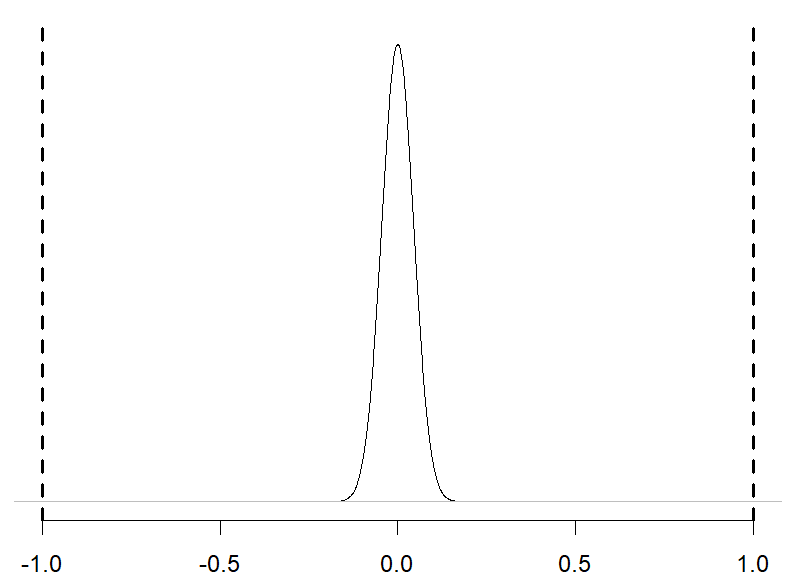
BONUS: The plot above may have given the impression that the distribution of rs is normal (i.e., Gaussian), but it’s actually not.

A normal distribution extends infinitely to both the left and right, but the plot above does NOT. In fact, it CANNOT.

This is because correlation coefficients are bounded by -1 and +1, which crushes the null distribution in toward 0.

You may be able to see this if we zoom our plot out to include those boundaries…

# Wider-View Plot
plot(density(sim_rs),xlim=c(-1,1),
     xlab='',ylab='',main='',yaxt='n',bty='n')
abline(v=c(-1,1),lwd=2,lty=2)

Okay, enough nerdy stuff for today…