Nov. 4, 2026

I’ve previously explained p-values and checked the accuracy of the explanation using R code.

Now, let’s do what I originally planned to do before getting side-tracked, which is to show how we can calculate our own p-values using calculus.

Most p-values are not directly calculated by the individuals using or reporting them. Instead, they appear “magically” in the output of the analysis, which is often run using a platform like R, Python, SPSS, Stata, or MS Excel.

But as explained in the last two posts, the p-value is simply the proportion of a null distribution that’s at least as extreme as the result we actually calculated.

Using that information, we can calculate our own p-values rather than relying on canned code or hidden procedures.

• This serves as a second check on whether our understanding of p-values holds up.
• It also serves as another confirmation that we understand the basic idea behind integration in calculus.

The “slicing approach” to calculus finds the area of a shape by slicing it into many thin strips, approximating the area of each, and then adding them all up.

The narrower each slice is, the more the resulting sum converges on the true area. Therefore, to get precisely the correct answer, the widths of our slices must collapse toward zero.

If we understand both of these concepts correctly, then we can do a quick check in R (or whatever programming language).

Let’s put this in a hiring context…

Suppose we’re conducting an adverse impact analysis for an employee selection process. We have two groups (let’s call them “Group 1” and “Group 2”), and we are examining the difference between their selection ratios (i.e., the proportions hired out of the totals that applied).

Imagine that we run some relevant calculations and find that the difference can be described by z = 2.20 in a standard normal distribution.

A p-value can tell us the probability of a result at least this extreme if the “true effect” is zero (i.e., if there’s hypothetically no real difference in hiring rates, beyond random noise).

This is equivalent to the area under the standard normal curve that lies beyond ±2.20 (in dark red below), expressed as a proportion of the total area under the curve…

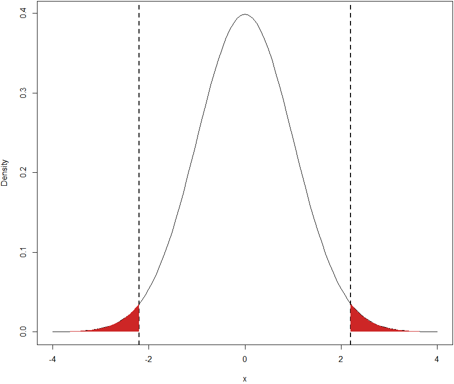
To calculate p using the slicing method, we will…

1. Slice up all the area under the curve more extreme than ±2.20
2. Approximate the area of each
3. Sum the areas

The purpose here is to demonstrate that our mental model of these concepts is accurate. We’ll do that by creating a digital representation of the concepts and then checking if it produces the correct results to some acceptable approximation.

First, let’s slice up the area under the curve more extreme than ±2.20…

> # 1. Identifying Slices
> slices=c(seq(-10,-2.2,by=1e-06),
+          seq(2.2,10,by=1e-06))

Because the area under the curve gets so small the further out you go, I’m only going to approximate this with the ranges z = -10 to -2.2 and z = 2.2 to 10.

Notice that this code specifies the slice width as an arbitrarily narrow value of 1e-06 = .000001. (The narrower we set it, the more precisely our approximation will match the true result.)

Next, we need to approximate the area of each slice. For this, we’ll treat the slices as rectangles with equal width and with heights equal to the vertical distances under the curve. (The areas aren’t really rectangles, but because the slices are so thin, the slight error is negligible.)

We already know the widths…

> # 2. Approximating Areas of Slices
> # 2a. Widths
> slice_width=1e-06

The slice height can be calculated using the probability density function for a normal curve, which is …

[1/√(2π)] ⋅ e^(-x²/2)

For example, we could manually calculate this for z = 2.5…

> (1/sqrt(2*pi))*exp(-2.5^2/2)
[1] 0.0175283

Or we could simply use a built-in function, like dnorm(), which gives the same result…

> dnorm(2.5)
[1] 0.0175283

Either way, let’s assign those slice heights…

> # 2b. Heights
> slice_height=dnorm(slices)

Cool. Next, because the area of a rectangle is simply Area = Base ⋅ Height, that’s our next step…

> # 2c. Slice Areas
> slice_areas=slice_width*slice_height

Finally, we sum these areas to get the full area under the curve more extreme than ±2.2 (i.e., the p-value)…

> # 3. Summing Approximated Slice Areas
> sum(slice_areas)
[1] 0.02780693

We can check this in multiple ways.

First, let’s see how this stacks up against the exact calculation using the pnorm() function…

> # Precise p-Value
> 2*pnorm(-2.2)
[1] 0.0278069

Clearly, our result matches the more precise calculation to several significant digits. This is more evidence that our understanding of p-values is correct.

Next, let’s check if our understanding of the slicing method is on-target. We can do this by using the integrate() function in R…

> 2*integrate(dnorm,2.2,10)$value
[1] 0.0278069

This matches our slicing approximation to several significant digits as well.

By the way, we could also integrate from ±2.2 to negative and positive infinity, which would cover both entire tails of the distribution…

> 2*integrate(dnorm,2.2,Inf)$value
[1] 0.0278069

Okay, it all worked out as expected. These demonstrations further support our belief that our mental models of both p-values and the slicing method calculus are on target.

Obviously, you wouldn’t actually calculate these things in this “manual” way in your own work or research. It’s super inefficient.

But that’s not the point. The purpose of exercises like these is to evaluate the extent to which you genuinely understand the concepts at a relatively deep level.

Once you do understand, then it’s almost irresponsible not to use more efficient code.

Understand, then automate.